Excel 2016

About Excel Chart

Method 1 - Add Secondary Axis to Combine Bar and Line Graph in Excel. STEPS Select the data range to use for the graph. In our case, we select the whole data range B5D10. Go to the Insert tab from the ribbon. Click on the Insert Column or Bar Chart drop-down menu, under the Charts category. Select the Clustered Column under the 2-D Column.We'll use the Clustered Column since the order

Tips The same technique can be used to plot a median For this, use the MEDIAN function instead of AVERAGE. Adding a target line or benchmark line in your graph is even simpler. Instead of a formula, enter your target values in the last column and insert the Clustered Column - Line combo chart as shown in this example. If none of the predefined combo charts suits your needs, select the

Predefined line and bar types that you can add to a chart. Depending on the chart type that you use, you can add one of the following lines or bars Series lines These lines connect the data series in 2-D stacked bar and column charts to emphasize the difference in measurement between each data series. Pie of pie and bar of pie charts display

Step 3 Create Bar Chart with Average Line. Next, highlight the cell range A1C13, then click the Insert tab along the top ribbon, then click Clustered Column within the Charts group. The following chart will be created Next, right click anywhere on the chart and then click Change Chart Type In the new window that appears, click Combo and

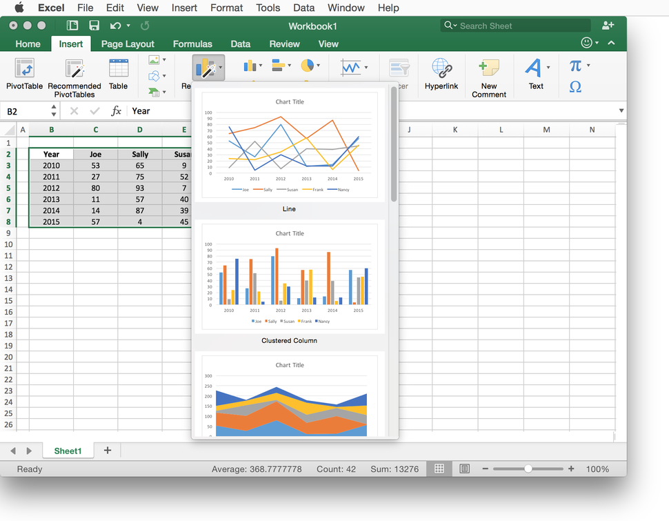
One of the best ways of visualizing data is through charts. Bar and line graphs are one of the most popular types of charts in Excel. You can easily convert excel tables into graphs or charts. Other popular graphs that you can create in Excel include pie charts, scatter graphs, histograms, and waterfall graphs. To

2. Now a bar chart is created in your worksheet as below screenshot shown. Select the specified bar you need to display as a line in the chart, and then click Design gt Change Chart Type. See screenshot 3. In the Change Chart Type dialog box, please select Clustered Column - Line in the Combo section under All Charts tab, and then click the

Add the real average values into the x field, and the dummy 'Average_y' values into the y field. Click OK and the average line will now be vertical across the chart. One more step though may be needed! Excel may add a bit of extra length to the secondary y axis, so your average line isn't quite matching the height of the chart.

Example 3 - Add a Line to a Bar Chart as the Target Line. Set up a number as the target value in the dataset and select the whole dataset. Create a bar chart. Right-click on the chart and select Change Chart Type. In the new window, go to Combo from the All Charts section and select Custom Combination. Press OK. You can see a line in the bar chart as the target line.

Learn how to add a vertical line to a horizontal bar chart in Excel. The tutorial walks through adding an Average value line to a new series on the graph. The horizontal bar chart is a great example of an easy to use graph type. Sometimes, though, it can be useful to call attention to a particular value or performance level, like an average

Creating a bar chart in Excel is straightforward, but adding a target line can seem a bit more challenging. This is a skill worth mastering because it provides a clear visual representation of your goals compared to your actual performance. Imagine you're trying to track sales against a monthly target. With a target line, you get a quick snapshot of how you're doing.